See also: FDT: Kevin’s Last Sketch 2019
Suppose our data is a stream of pairs {IP address, User ID} and we want to identify the IP addresses that have the most distinct User IDs. Or conversely, we would like to identify the User IDs that have the most distinct IP addresses. This is a common challenge in the analysis of big data and the FDT sketch helps solve this problem using probabilistic techniques.
More generally, given a multiset of tuples with N dimensions {d1,d2, d3, …, dN}, and a primary subset of dimensions M < N, our task is to identify the combinations of M subset dimensions that have the most frequent number of distinct combinations of the N - M non-primary dimensions.
Suppose we have a stream of 160 items where the stream consists of four item types: A, B, C, and D. If the distribution of occurrences was shared equally across the four items each would occur exactly 40 times or 25% of the total distribution of 160 items. Thus the equally distributed (or fair share) threshold would be 25% or as a fraction 0.25.
We define Most Frequent items as those that consume more than the fair share threshold of the total occurrences (also called the weight) of the entire stream.
Suppose we have a stream of 160 items where the stream consists of four item types: A, B, C, and D, which have the following frequency distribution:
We would declare that A is the most frequent and B is the next most frequent. We would not declare C and D in a list of most frequent items since their respective frequencies are below the threshold of 40 or 25%.
If all items occurred with a frequency of 40, we could not declare any item as most frequent. Requesting a list of the “Top 4” items could be a list of the 4 items in any random order, or a list of zero items, depending on policy.
When a stream becomes too large with too many different item types to efficiently process exacty we must turn to statistical methods to estimate the most frequent items. The returned list of “most frequent items” will have an associated “estimated frequency” that has an error component that is a random variable. The RSE is a measure of the width of the error distribution of this component and computed similarly to how a Standard Deviation is computed. It is relative to the estimated frequency in that the standard width of the error distribution can be computed as estimate * (1 + RSE) and estimate * (1 - RSE).
We define a specific combination of the M primary dimensions as a Primary Key and all combinations of the M primary dimensions as the set of Primary Keys.
We define the set of all combinations of N-M non-primary dimensions associated with a single primary key as a Group.
For example, assume N = 3, M = 2, where the set of Primary Keys are defined by {d1, d2}. After populating the sketch with a stream of tuples all of size N = 3, we wish to identify the Primary Keys that have the most frequent number of distinct occurrences of {d3}. Equivalently, we want to identify the Primary Keys with the largest Groups.
Alternatively, if we choose the Primary Key as {d1}, then we can identify the {d1}s that have the largest groups of {d2, d3}. The choice of which dimensions to choose for the Primary Keys is performed in a post-processing phase after the sketch has been populated. Thus, multiple queries can be performed against the populated sketch with different selections of Primary Keys.
An important caveat is that if the distribution is too flat, there may not be any “most frequent” combinations of the primary keys above the threshold. Also, if one primary key is too dominant, the sketch may be able to only report on the single most frequent primary key combination, which means the possible existance of false negatives.
In this implementation the input tuples presented to the sketch are string arrays.
Let’s leverage the challenge at the beginning to create a concrete example. Let’s assume N = 2 and let d1 := IP address, and d2 := User ID.
If we choose {d1} as the Primary Keys, then the sketch will allow us to identify the IP addresses that have the largest populations of distinct User IDs.
Conversely, if we choose {d2} as the Primary Keys, the sketch will allow us to identify the User IDs with the largest populations of distinct IP addresses.
Let’s set the threshold to 0.01 (1%) and the RSE to 0.05 (5%). This is telling the sketch to size itself such that items with distinct frequency counts greater than 1% of the total distinct population will be detectable and have a distinct frequency estimation error of less than or equal to 5% with 86% confidence.
//Construct the sketch
FdtSketch sketch = new FdtSketch(0.01, 0.05);
Assume the incoming data is a stream of {IP address, User ID} pairs:
//Populate
while (inputStream.hasRemainingItems()) {
  String[] in = new String[] {Pair.IPaddress, Pair.userID};
  sketch(in);
}
We are done populating the sketch, now we post process the data in the sketch:
int[] priKeyIndices = new int[] {0}; //identifies the IP address as the primary key
int numStdDev = 2; //for 95% confidence intervals
int limit = 20; //list only the top 20 groups
char sep = '|'; //the separator character for the group dimensions as strings
List<Group> list = sketch.getResult(priKeyIndices, limit, numStdDev, sep);
System.out.println(Group.getHeader())
Iterator<Group> itr = list.iterator()
while (itr.hasNext()) {
  System.out.println(itr.next())
}
If we want the converse relation we assign the UserID as the primary key. Note that we do not have to repopulate the sketch!
int[] priKeyIndices = new int[] {1}; //identifies the User ID as the primary key
...
When the Group is printed as a string, it will output seven columns as follows:
Count: This is the number of retained occurrences in the sketch that belong to this group.
Est This is the sketch’s estimate of the distinct cardinality of this group based on the Count and the sketche’s internal state of Theta.
UB: The Upper Bound of the confidence interval based on the given numStdDev.
LB: The Lower Bound of the confidence interval based on the given numStdDev.
Fraction: The fractional proportion of the cardinality of the entire sketch that this group represents.
RSE: The estimated RSE of this group based on the properties of this group and the internal properties of this sketch.
PriKey: The string identifying this group.
Note: the code for the following study can be found in the characterization repository here and the configuration file can be found here. A login to GitHub will be required.
In order to study the error behavior of this sketch a power-law distribution with a slope of -1 was created. The head of the distribution was a single item with a cardinality of 16384, and the tail of the distribution was 16384 items each with a cardinality of one. All the points in between were items that have multiplicities and cardinalities that would fall on a straight line plotted on a Log-X, Log-Y graph. This generated an input stream of about 850K (Key, value) pairs, which was input into the sketch and is considered one trial. The sketch was constructed with a target threshold of 1% and a target RSE of 5%.
Twenty such trials were run and the error distribution quantiles of the results were computed and is shown in the following graph.
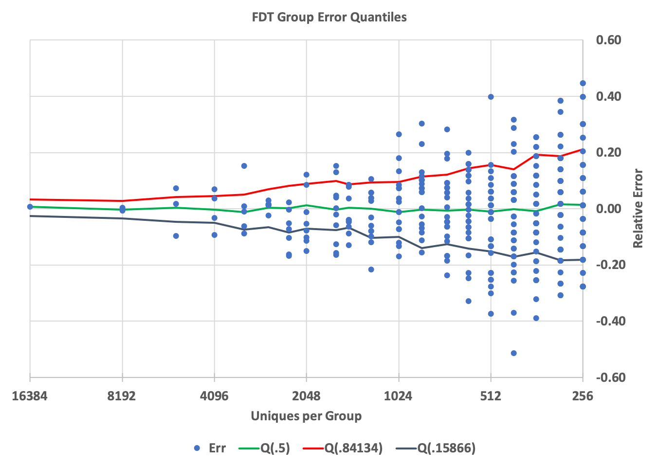
The X-axis is the true cardinality. Of the nearly 24K groups captured by the sketch of the input stream of over 100K groups this graph is a view of the top 500, which is more than enough to demonstrate the error behavior.
The Y-axis is the relative error.
The blue dots represent the error of a single group from the top 500 groups. Not all of the top 500 groups are shown on the graph as number of them had true cardinalities of less than 256. Also many of the dots represent multiple groups since groups with the same Count and the same true cardinality will result in the same exact computed error, thus plotted at the same exact point.
The red line is the contour of the quantile(0.84) points of the error distribution at each point along the X-axis. This quantile contour would be equivalent to the +1 standard deviation from the mean of a Gaussian distribution. But since these are quantile measurements of the actual error distribution there is no assumption whatsoever that the error distribution is Gaussian. It is just a convenient reference contour. Similarly the black line is the contour of the quantile(0.159), which corresponds to the -1 standard deviation from the mean. Between these two contours would represent 68% of the distribution (or 68% confidence), which is equivalent to saying within +/- 1 standard deviation of the mean (if it were Gaussian). The green line is the contour of the medians (quantile(0.5)).
The following table is the list of the top 10 results from just one of the trials. The Group class was extended to include more columns at the end which were useful for this study. (This was easy to do and does not require any special access.)
Count         Est          UB          LB      Thresh         RSE      PriKey   xG      yU         Err
 1338    16511.86    16957.05    16078.18    0.019521    0.026962   1,1,16384    1   16384    0.007804
  666     8218.91     8536.72     7912.67    0.009717    0.038668    2,1,8192    2    8192    0.003285
  660     8144.87     8461.30     7840.01    0.009629    0.038850    2,2,8192    2    8192   -0.005754
  475     5861.83     6132.21     5603.08    0.006930    0.046124    3,1,5461    3    5461    0.073400
  450     5553.32     5816.82     5301.44    0.006565    0.047449    3,2,5461    3    5461    0.016905
  400     4936.28     5185.44     4698.76    0.005836    0.050475    3,3,5461    3    5461   -0.096085
  355     4380.95     4616.42     4157.14    0.005179    0.053748    4,2,4096    4    4096    0.069568
  344     4245.20     4477.19     4024.87    0.005019    0.054648    4,1,4096    4    4096    0.036426
  321     3961.37     4185.90     3748.50    0.004683    0.056681    4,3,4096    4    4096   -0.032870
  306     3776.26     3995.79     3568.40    0.004464    0.058134    5,5,3277    5    3277    0.152351
The blue dot on the very left represents the single item with the largest cardinality. As you can see from the table, it’s estimation error is quite small (about 0.78%). At this point the +/- 1 S.D. contours are at about +3.4% and -2.5% and the median is about 0.78%
As you follow the graph to the right you are observing the error distribution as the cardinalities get smaller. Smaller groups have fewer samples from the sketch thus their estimation error will, of course, grow larger. What this graph demonstrates is the the error properties are well behaved and what one would expect from this sketch.

