Accuracy Plots

Accuracy of the Theta: QuickSelect Sketch Family

A QuickSelect Sketch, which is the default sketch family, can be constructed with code similar to:

int k = 4096;                        //the accuracy and size are a function of k
UpdateSketch sketch = UpdateSketch.builder().build(k);  //build an empty sketch

long u = 1000000;                    //The number of uniques fed to the sketch
for (int i=0; i<u; i++) {            //A simple loop for illustration
  sketch.update(i);                  //Update the sketch
}

double est = sketch.getEstimate();   //get the estimate of u

sketch.rebuild(); // An optional rebuild to reduce the sketch size to k. This ensures order insensitivity. 

// Get the upper and lower bounds (optional). 

double ub = sketch.getUpperBound(1); //+1 standard deviation from the estimate
double lb = sketch.getLowerBound(1); //-1 standard deviation from the estimate

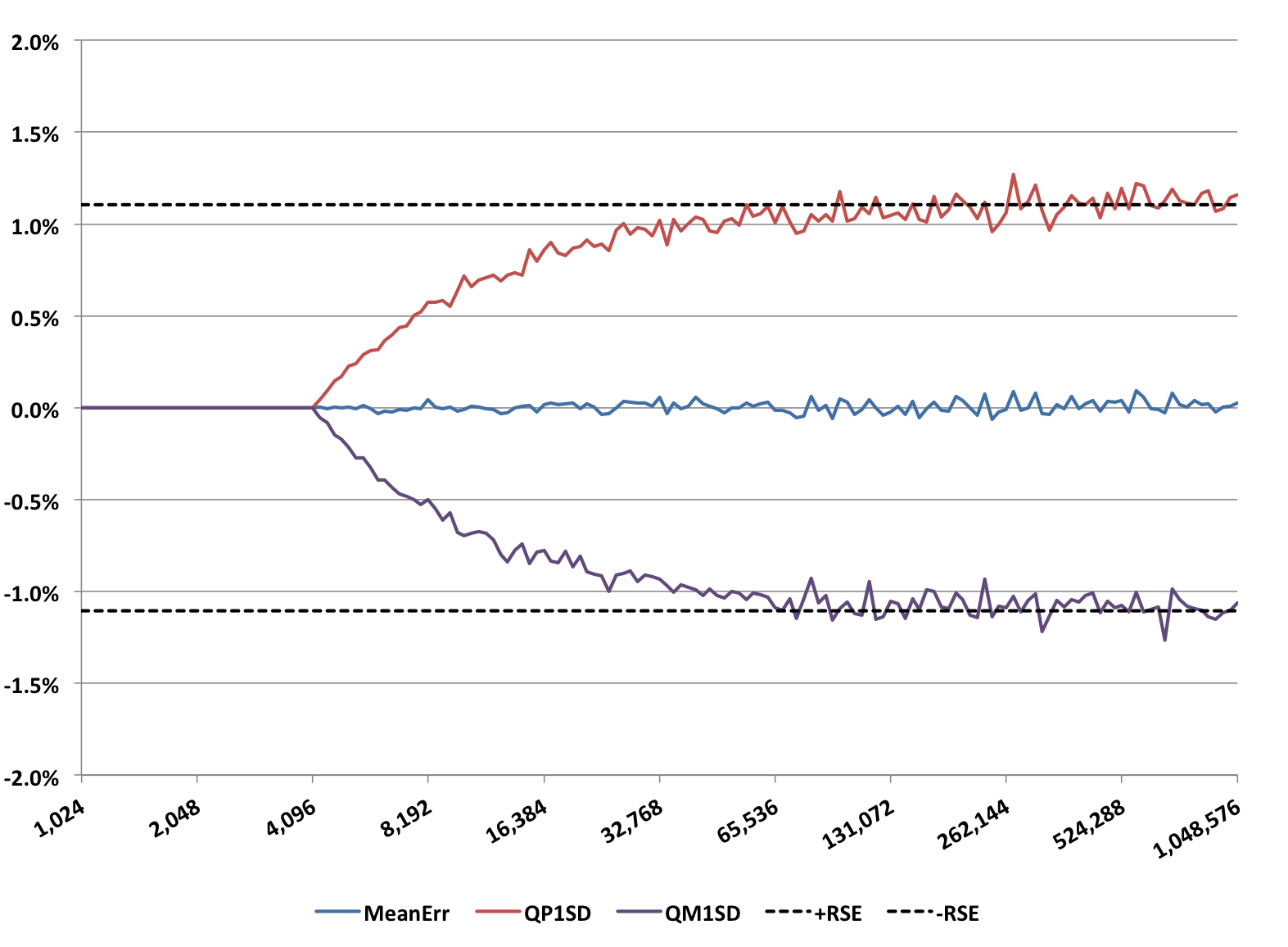
The accuracy behavior of this QuickSelect Sketch (the default, with no rebuild) will be similar to the following graph:

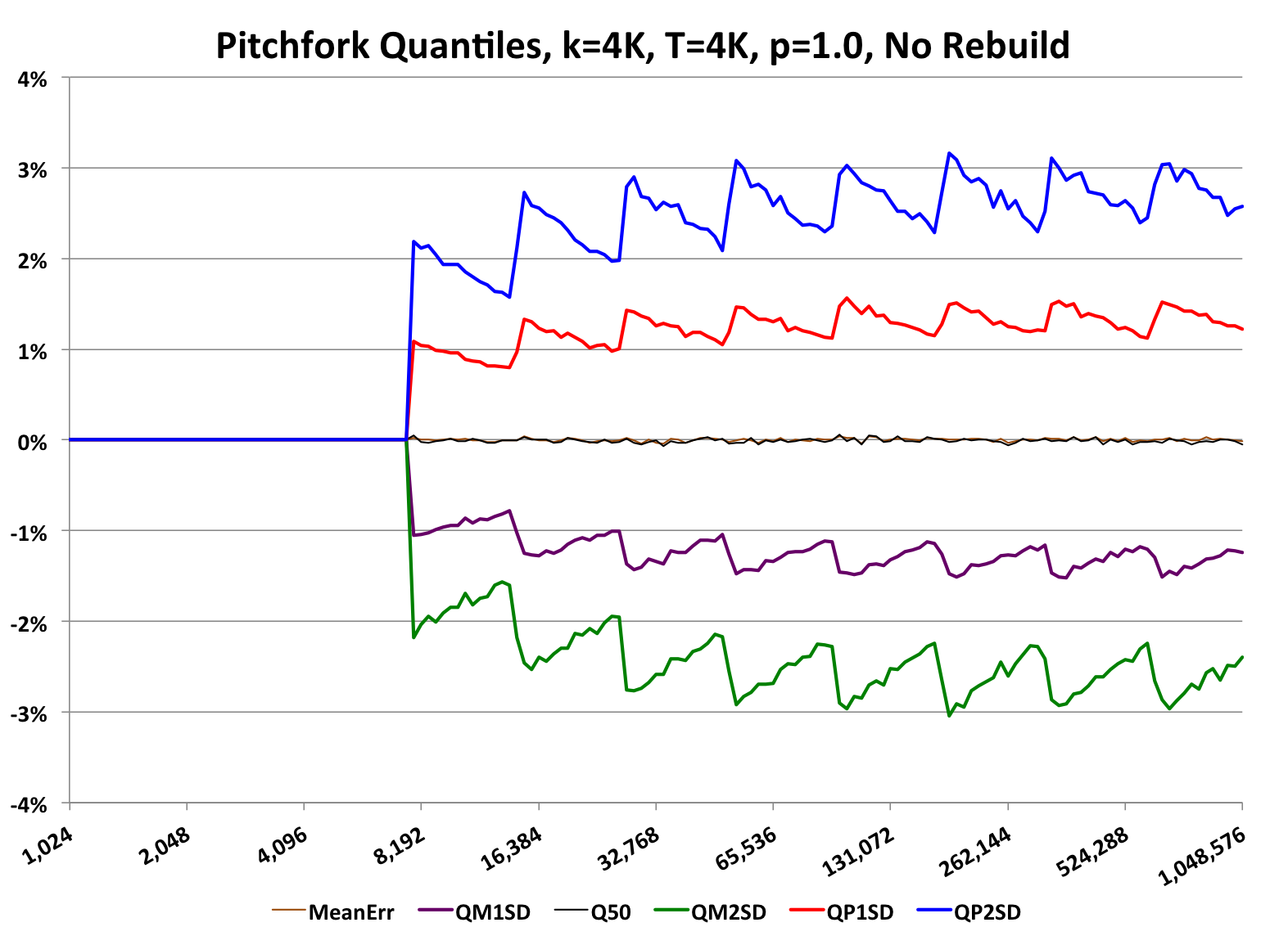
This type of graph is called a “pitchfork”, which is used throughout this documentation to characterize the accuracy of the various sketches.

Pitchfork graphs have these common characteristics:

• The x-axis is Log(base 2) and represents the number of unique values fed into a sketch.
  • Points along the x-axis are evenly spaced along the log axis with the same number of Points Per Octave (PPO) for every multiple of 2 along the x-axis. This means that the plotted x values form an exponential series of the form 2^(gi/PPO), where gi is the Generating Index for a particular point on the x-axis.
  • A Trial is the estimation result of a single sketch fed x unique values.
  • A Trial Set is the set of results of runing T independent trials at x.
• The y-axis measures the Relative Error (RE) of result estimates returned by the sketches in the trials, where RE = MeasuredValue/TrueValue -1 and is plotted as a percent.
  • An imaginary line drawn vertically from each x-axis point represents the range of error values that result from the Trial Set. However, not all of the error values from all the trials are plotted. Instead, for each Trial Set, the result error values are sorted and then selected quantiles are chosen and then only those y-axis values are plotted.
  • Connecting the plotted points with the same quantiles form the lines of the graph
• The plotted lines on these graphs are actually the lines of constant quantiles of the distributions of error measured at each x-axis point on the graph.
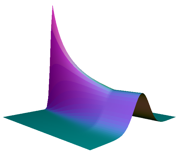• These pitchfork graphs are just two dimensional views of a three-dimensional probability surface that would look something like this: . The cross-sectional slice of this surface is approximately Gaussian like this graph 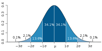, which has the +/- 1, 2 and 3 standard deviation points on the x-axis marked and the corresponding areas under the curve that represent the associated confidence levels.
• All the pitchfork graphs in this section were generated using the utilities located in the the datasketches-characterization repository.

The specifics of the above pitchfork graph:

• The sketch type is the Heap QuickSelect Sketch, which is the default Theta UpdateSketch.
• The sketch was configured with k = 4096.
• The x-axis varies from 1024 (2^10) uniques per sketch to 1,048,576 (2^20) uniques per sketch.
• PPO = 16.
• Trials, T = 4096.
• Wavy colored lines:
  • The black wavy line in the center (at Y = 0%) represents the median of the distribution of error values. The median sits on top of the mean, which is brown and hard to see. The fact that the mean and median are at zero validates the assertion that the estimates from the sketch are unbiased.
  • The red wavy line is the connected quantiles at +1 Relative Standard Error (RSE), which means ~15.87% of the trial results are above that line.
  • The blue wavy line is the connected quantiles at +2 RSE, which means ~2.3% of the trial results are above that line.
  • The purple wavy line is the connected quantiles at -1 RSE, which means ~15.87% of the trial results are below that line.
  • The green wavy line is the connected quantiles at -2 RSE, which means ~2.3% of the trial results are below that line.

This particular graph also illustrates some other subtle points about this particular sketch.

• The saw-toothed variation in the overall shaped is due to the fact that the QuickSelect sketch only updates its internal theta when the hash table fills up, which occurs when the hash table reaches 15k/8 (note that the estimation starts at almost 8K), at which point the sketch uses the QuickSelect algorithm to find the (k + 1)^th order statistic from the cache, assigns this value to theta, discards all values above theta, and rebuilds the hash table.
• Because the number of valid points nearly reaches 2k values means that the Relative Error of the sketch nearly reaches 1/sqrt(2k).

If the user does not want the sketch ever to exceed k values, then there is an optional rebuild method (see code snippet above) that can be used. This would result in the following graph:

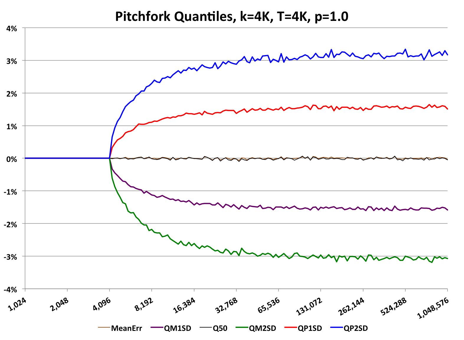
Because of the extra rebuild at the end the full cycle time of the sketch is a little slower and the average accuracy is a little less than without the rebuild. This is a tradeoff the user can choose to use or not.

The quantiles for both +/- 1 RSE and +/- 2 RSE establishes the bounds for the 68% and 95.4% confidence levels respectfully.

Accuracy of Set Intersections & Differences

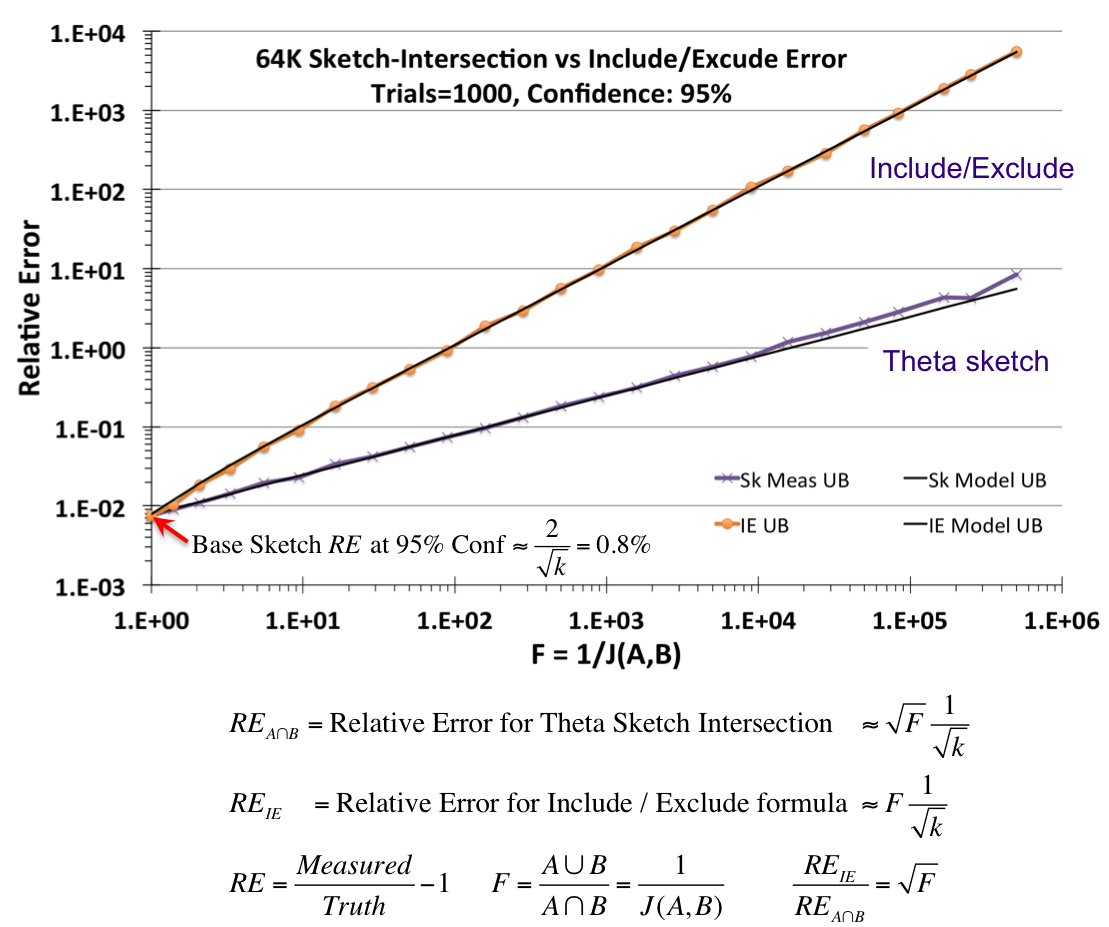
The above diagram was created using two Theta Sketches, A and B, with nominal entries size of 64K. The number of unique items presented to the two sketches was quite large, but the ratio of the number of uniques presented to the two sketches varies along the X-axis in a special way.

The X-axis is the inverse Jaccard ratio, where the Jaccard is defined as the intersection divided by the union of two sets. Thus, the X-axis is defined as 1/J(A,B) = (A∪B)/(A∩B).

Given any two sets, A and B, the intersection can be defined from the set theoretic Include/Exclude formula (A∩B) = A + B - (A∪B). Unfortunately, for stochastic processes, each of these terms have random error components that always add. The upper line and orange points represent the resulting error of an intersection using the Include/Exclude formula. The lower black line and purple “X” points represent the resulting error from an intersection using the Theta sketch set operations, which can be orders-of-magnitude better than the naive application of the Include/Exclude relation.

Set intersections and differences can have considerably more relative error than a base Theta sketch fed directly with data. Be cautious about situations where the result of an intersection (or difference) is orders-of-magnitude smaller than the union of the two arguments. Always query the getUpperBound() and getLowerBound() methods as these funtions are specifically designed to give you conservative estimates of the possible range of values where the true answer lies.

Theta sketches retain only a small sample of the input streams that that they see. When you perform an intersection it reduces that small sample to an even smaller set, possibly zero! And as you might guess, extracting useful information about your input streams with zero samples is rather difficult:

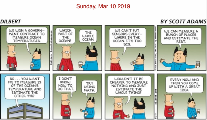
Successive intersections will quickly reduce your number of samples available to estimate from and thus will dramatically increase the error. Also attempting to intersect one sketch from a large cardinality set with another sketch from a very small cardinality set will also increase your error (see the graph above).

So what can you do?

• Organize your intersections (and AnotB ops) to be performed as the very last step. For example, instead of AU(B^C) use (AUB)^(AUC). This keeps the internal sample set as large as possible until the very end.
• If you know which streams have large cardinality, use large sketches for these sketches. Internally we use sketches of 2^20 for our large cardinality streams (there is generally only a few of them) and then 2^14 for everything else.
• Always query the resulting sketch from a set expression to obtain the upper and lower bounds. This will tell you right away what your error confidence interval is.

Accuracy of the Theta: Alpha Sketch Family

Another major sketch family is the Alpha Sketch, which leverage the “HIP” estimator. Its pitchfork graph looks like the following:

This sketch was also configured with a size of 4K entries, otherwise the defaults. The wavy lines have the same interpretation as the wavy lines for the QuickSelect Sketch above. The short-dashed reference lines are computed at plus and minus 1/sqrt(2k). The Alpha Sketch is about 30% more accurate than the QuickSelect Sketch with rebuild for the same value of k. However, this improved accuracy can only be obtained when getEstimate() is directly called from the Alpha Sketch. After compacting to a Compact Sketch or after any set operation, the accuracy falls back to the standard 1/sqrt(k).