Theta Family Update Speed

Resize Factor = X1

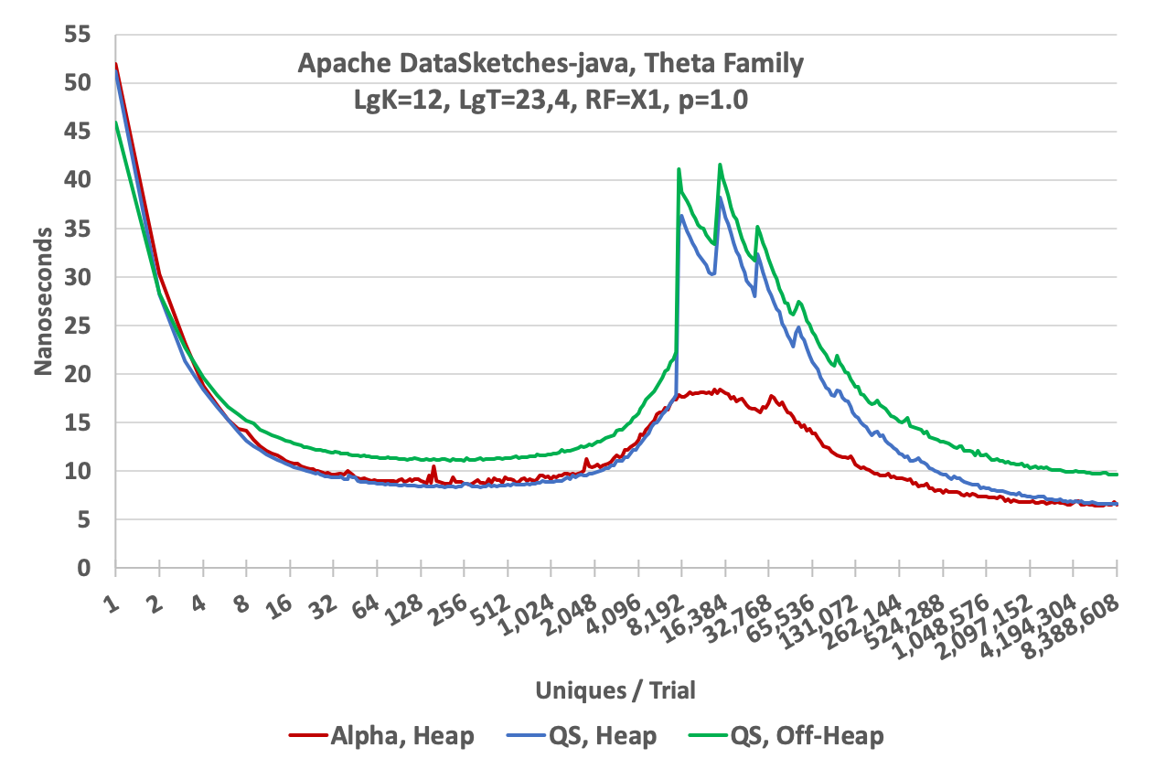
The following graph illustrates the update speed of 3 different sketches from the library: the Heap QuickSelect (QS) Sketch, the Off-Heap QuickSelect Sketch, and the Heap Alpha Sketch. The X-axis is the number of unique values presented to a sketch. The Y-axis is the average time to perform an update. It is computed as the total time to update X-uniques, divided by X-uniques.

The high values on the left are due to Java overhead and JVM warmup. The spikes starting at about 4K uniques are due to the internal hashtable filling up and forcing an internal hashtable rebuild, which also reduces theta. For this plot the sketches were configured with k = 4096. The sawtooth peaks on the QuickSelect curves represent successive rebuilds. The downward slope on the right side of the largest spike is the sketch speeding up because it is rejecting more and more incoming hash values due to the continued reduction in the value of theta. The Alpha sketch (in red) uses a more advanced hashtable update algorithm that defers the first rebuild until after theta has started decreasing. This is the little spike just to the right of the local maximum (at about 16K) of the curve. As the number of uniques continue to increase the update speed of the sketch becomes asymptotic to the speed of the hash function itself, which is about 6 nanoseconds.

• The Heap Alpha Sketch (red) is the fastest sketch of the Theta family and primarily focused on real-time streaming environments and operates only on the Java heap. Performing an “average” over all the test points from about 8 to 8 million uniques, the Alpha sketch update rate averages about 100 million updates per second.
• The Heap QuickSelect sketch (blue) is next fastest. It averages about 81 million updates per second.
• The Off-Heap QuickSelect sketch (green) runs in direct, native memory and averages about 63 million updates per second.
• The notations in the second line of the title are abbreviations as follows:
  • LgK = 12 : The sketch was configured with K = 2^12 or 4096 nominal hash values.
  • LgT = 23,4 : The test harness was configured to start with 2^23 trials on the left and logarithmically decrease the trials as the number of uniques increase down to 2^4 trials on the right.
  • RF = X1 : Resize Factor = 1. The sketch was configured to start at maximum possible size in memory. This means there is no need for the sketch to request (allocate) more memory for the life of the sketch. This is the overall fastest configuration at the expense of allocating the maximum memory upfront. Other RF values are discussed below. This has no impact on space required when serializing the sketch in compact mode.

Resize Factors = X1, X2 and X8

To illustrate how the the optional Resize Factor affects performance refer to the following graph. All three plots were generated using the Heap QuickSelect Sketch but with different Resize Factors.

• The blue curve is the same as the blue curve in the graph at the top of this page. It was generated with ResizeFactor = X1, which means the sketch cache was initially created at full size, thus there is no resizing of the cache during the life of the sketch. (There will be rebuilding but no resizing.)
• The red curve is the same sketch but configured with ResizeFactor = X2, which means the sketch cache is initially created at a small size (enough for about 16 entries), and then when the sketch needs more space for the cache, it is resized by a factor of 2. Each of these resize events are clearly seen in the curve as sawtooth spikes where the sketch must pause, allocate a larger cache and reconstruct the hashtable. These spikes fall at factors of 2 along the X-axis (with the exception of the last interval, which is a factor of 4 for reasons too complicated to explain here.)
• The green curve is the same sketch but configured with ResizeFactor = X8. An RF = X4 is also available but not shown.

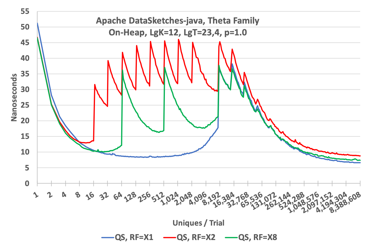
As one would expect the overall speed of the RF = X2 sketch is slower than the RF = X1 sketch and the RF = X8 sketch is inbetween due to the amount of time the sketch spends in resizing the cache.

The tradeoff here is the classic memory size versus speed. Suppose you have millions of sketches that need to be allocated and your input data is highly skewed (as is often the case). Most of the sketches will only have a few entries and only a small fraction of all the sketches will actually go into estimation mode and require a full-sized cache. The Resize Factor option allows a memory allocation that would be orders of magnitude smaller than would be required if all the sketches had to be allocated at full size. The default Resize Factor is X8, which is a nice compromise for many environments.

How these graphs were generated

The goal of these measurements was to measure the limits of how fast these sketches could update data from a continuous data stream not limited by system overhead, string or array processing. In order to remove random noise from the plots, each point on the graph represents an average of many trials. For the low end of the graph the number of trials per point is 2^23 or 8M trials per point. At the high end, at 8 million uniques per trial, the number of trials per point is 2^4 or 16.

It needs to be pointed out that these tests were designed to measure the maximum update speed under ideal conditions so “your mileage may vary”! Very few systems would actually be able to feed a single sketch at this rate so these plots represent an upper bound of performance, and not as realistic update rates in more complex systems environments. Nonetheless, this demonstrates that the sketches would consume very little of an overall system’s budget for updating, if there was one, and are quite suitable for real-time streams.

The graphs on this page were generated using the utilities in the Characterization Repository. There is some more documentation with the code on using these tools if you wish to re-run these characterization tests yourself.

Measurement System

Model Name: Apple MacBook Pro
Model Identifier: MacBookPro11,3
Processor Name: Intel Core i7
Processor Speed: 2.5 GHz
Number of Processors: 1
Total Number of Cores: 4
L2 Cache (per Core): 256 KB
L3 Cache: 6 MB
Memory: 16 GB 1600 MHz DDR3