Package: org.apache.datasketches.quantiles
This is a stochastic streaming sketch that enables near-real time analysis of the approximate distribution of comparable values from a very large stream in a single pass. The analysis is obtained using a getQuantiles() function or its inverse functions, the Probability Mass Function, getPMF(), and the Cumulative Distribution Function, getCDF().
Consider this real data example of a stream of 230 million time-spent events collected from one our systems for a period of just 30 minutes. Each event records the amount of time in milliseconds that a user spends on a web page before moving to a different web page by taking some action, such as a click.
An exact, brute-force approach to computing an arbitrary quantile would require creating a sorted list all 230 million values and then choosing an index into this list for the desired quantile. This index is the absolute rank of the values in the sorted list and in this case would vary from zero to 230 million. The value at rank = 115M is the median or 50th percentile; normalized Rank is computed by dividing the absolute rank by the size of the list, which produces a fraction between zero and one. Quantiles are values corresponding to a normalized rank. Thus, the median value = quantile(0.5). The quantile(0.95) is the value from the stream at the absolute rank (index) position (0.95) X 230M, which means only 5% of all the values from the stream are equal to or larger than this value.
The relevant pseudo-code snippets would look something like this:
int k = 256; //256 gives < 1% normalized rank error
UpdateDoublesSketch sketch = DoublesSketch.builder().setK(k).build();

while ( remainingValuesExist ) { //stream in all the values, one by one
  sketch.update(nextValue());
}

//Query the sketch with a sorted array of 101 normalized ranks from zero to one:

double[] normRanks = {0, .01, .02, ... , .99, 1.0}; // Percentiles
double[] values = sketch.getQuantiles(normRanks); //result array of 101 values.
When these values are plotted against the normalized ranks we get something like this:
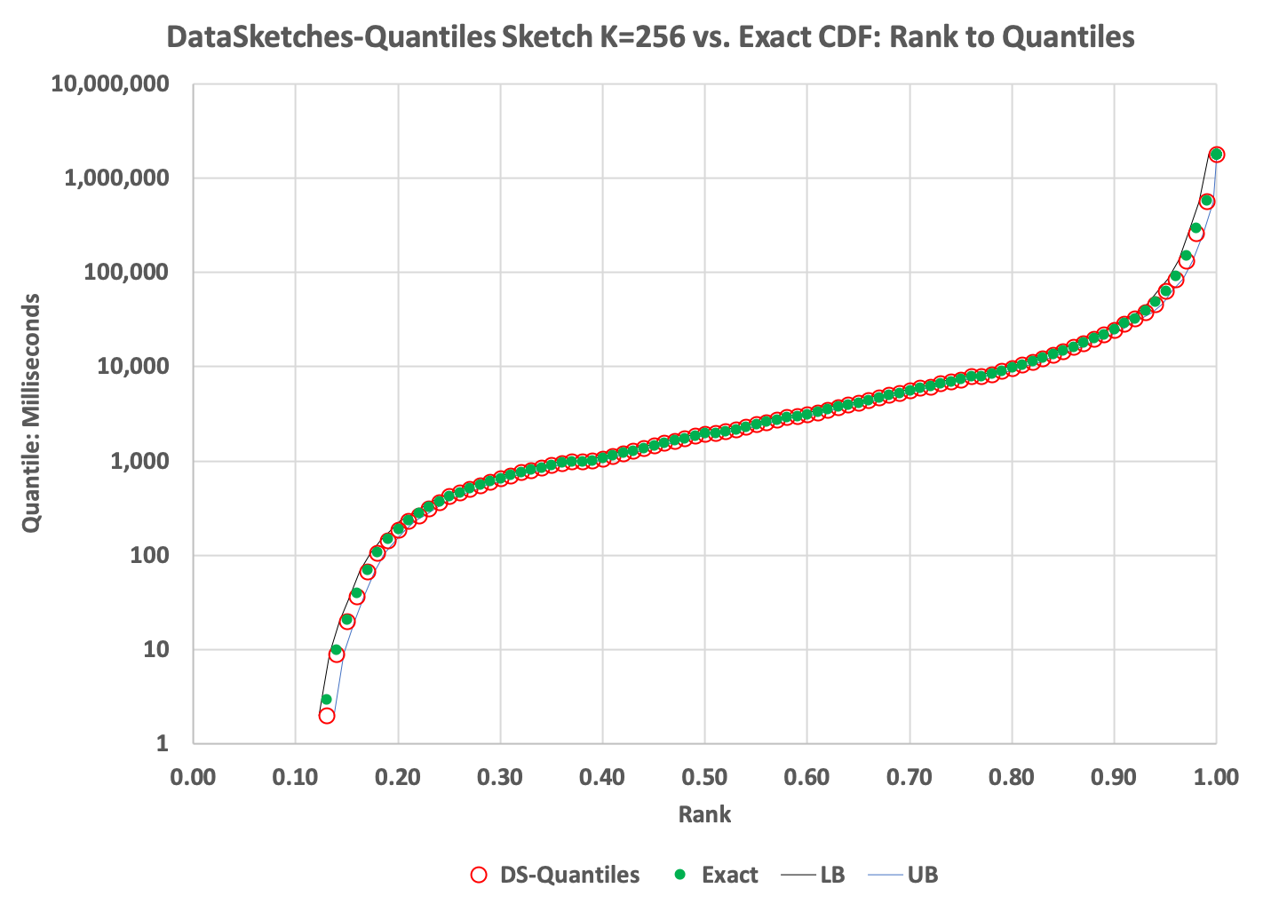
In this plot the green dots are the quantiles computed exactly and the red circles are the results from the quantiles sketch. The two curves on either side of these points represent the upper and lower bounds returned from the sketch.
This reveals a great deal about the distribution of values in the stream. Just reading from the graph, the median is about 2000 milliseconds and the 90th percentile is about 25,000 and so on. One can also query the min and max values seen by the sketch. By observing the results of the quantiles query, it is not too difficult to create a set of split points for a histogram plot.
In this case the values ranged from one to 1.8 million, which is a little over 6 orders-of-magnitude. (There are zero values in the raw data, which often happens, but they can be ignored in this analysis.) In order to plot such a large dynamic range I used a log X-axis and a plot resolution of 5 points per factor of 10. Then I computed 36 equally spaced (on the log axis) split points with values from 1.0 to 1E7. These 36 split points are then provided to the getPMF() function:
double[] splitpoints = {1.00, 1.58, ... , 6.3E6, 1E7};
double[] pmf = sketch.getPMF(splitpoints);
The following histogram is plotted by multiplying all the pmf values by getN(), which is the total number of events seen by the sketch (230M). The getCDF(…) works similarly, but produces the cumulative distribution instead.
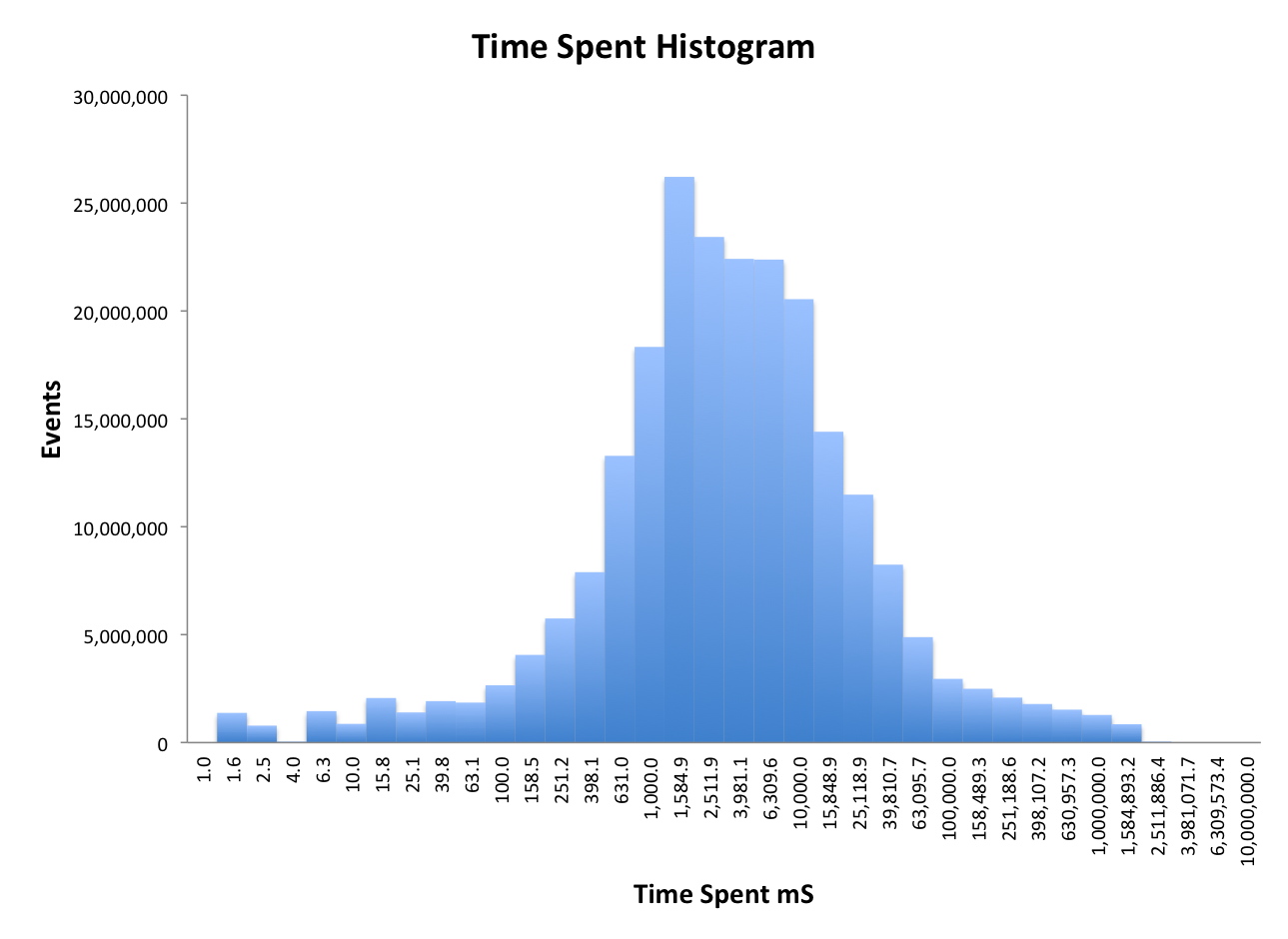
Now for some fun! For those of you that recognize the shape of this distribution as
looking remarkably similar to the Normal (Gaussian) Distribution, you are close, but no cigar!
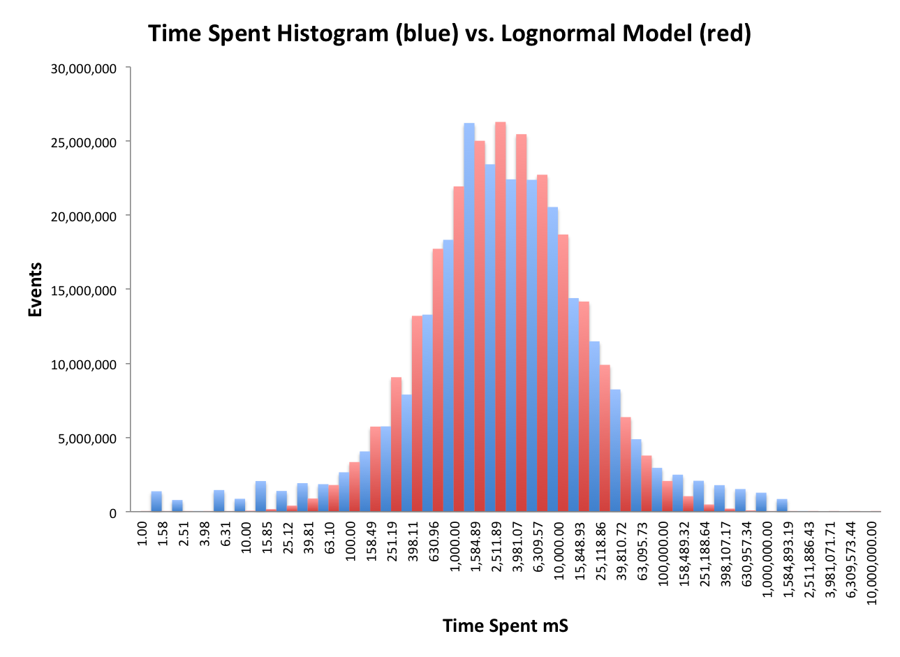
This data is plotted on a logarithmic axis so it is actually close to a Lognormal Distribution.
The following plot shows a mathematically generated Lognormal model in red,
and the actual data distribution in blue as before.
They are remarkably close within about 2 standard deviations on the log axis, but the tails are
way off.
Code examples are best gleaned from the test code that exercises all the various capabilities of the sketch. Here are some brief snippets, simpler than the above graphs, to get you started.
UpdateDoublesSketch qs = DoublesSketch.builder().build(); //default k = 128

for (int i=0; i < 1000000; i++) { //stream length is generally unknown
  qs.update(i); //load the sketch
}

double median = qs.getQuantile(0.5);
double topQuartile = qs.getQuantile(0.75);
System.out.println("Median = " + median);
System.out.println("75%ile = " + topQuartile);

/* Output similar to
Median = 500087.0
75%ile = 749747.0
*/
UpdateDoublesSketch qs = DoublesSketch.builder().build(); //default k = 128

for (int i=0; i < 1000000; i++) { //stream length is generally unknown
  qs.update(i); //load the sketch
}

//create a histogram
long n = qs.getN();
double[] splitPoints = {100000, 500000, 900000};

double[] fractionalRanks = qs.getPMF(splitPoints);
int bins = fractionalRanks.length;

double freq;
for (int i=0; i < bins-1; i++) {
  freq = fractionalRanks[i] * n;
  System.out.println(freq + " < "+splitPoints[i]);
}
freq = fractionalRanks[bins-1] * n;
System.out.println(freq + " >= "+ splitPoints[bins-2]);

/* Output similar to
98304.0  <  100000.0
401408.0 <  500000.0
400384.0 <  900000.0
99904.0  >= 900000.0
*/
UpdateDoublesSketch qs1 = DoublesSketch.builder().build(); //default k = 128
UpdateDoublesSketch qs2 = DoublesSketch.builder().build();
long size = 1000000; //generally unknown
for (int i=0; i < size; i++) { //update each value into the sketch
  qs1.update(i);
  qs2.update(i + 1000000);
}

Union union = Union.builder.build(); //creates a virgin Union
union.update(qs1);
union.update(qs2);

DoublesSketch qs3 = union.getResult();
System.out.println(qs3.toString()); //Primarily for debugging

/* Output similar to
### HeapQuantilesSketch SUMMARY:
   K                            : 128
   N                            : 2,000,000
   Seed                         : 0
   BaseBufferCount              : 128
   CombinedBufferAllocatedCount : 1,920
   Total Levels                 : 13
   Valid Levels                 : 6
   Level Bit Pattern            : 1111010000100
   Valid Samples                : 896
   Buffer Storage Bytes         : 15,360
   Preamble Bytes               : 36
   Normalized Rank Error        : 1.725%
   Min Value                    : 0.000
   Max Value                    : 1,999,999.000
### END SKETCH SUMMARY
*/
Any item type that is comparable, or for which you can create a Comparator, can also be analyzed by extending the abstract generic classes for that particular item.
Suppose you have a massive number of comparable MyItems that you wish to partition in to 10 equal parts for more efficient downstream processing. The task is to figure out how to equally partition your data.
First you build a comparator for MyItem:
public class MyComparator implements java.util.Comparator<MyItem> {
    @Override
    public int compare(MyItem item1, MyItem item2) {
        //compute equivalent to ...
        return (item1 < item2)? -1 : (item1 > item2)? 1 : 0;
    }
}
In distributed or multi-JVM environments you will also need to extend the ArrayOfItemsSerDe base class. Serialization and deserialization is required to move sketch images across JVMs. The methods in this class are called by the sketch toByteArray() and sketch constructor as necessary.
import org.apache.datasketches.ArrayOfItemsSerDe;
import org.apache.datasketches.memory.Memory;

public class ArrayOfMyItemsSerDe extends ArrayOfItemsSerDe<MyItem> {

  @Override
  public byte[] serializeToByteArray(MyItem[] items) {
    byte[] byteArr = // hopefully fast and efficient :)
    return byteArr;
  }

  @Override
  public MyItem[] deserializeFromMemory(Memory mem, int numItems) {
     //Memory is similar to ByteBuffer, but much more flexible
     // see org.apache.datasketches.memory
     MyItem[] myItemArr = new MyItem[numItems];
     for ( int i = 0; i < numItems; i++ ) {
       //extract each item from mem. See org.apache.datasketches.ArrayOfStringsSerDe example.
       MyItem item = //...
       myItemArr[i] = item;
     }
     return myItemArr;
  }
}
You are ready to feed all of MyItems into the sketch:
import org.apache.datasketches.quantiles.ItemsSketch;

ItemsSketch<MyItem> sketch = ItemsSketch.getInstance(128, new MyComparator());
while ( remainingItemsExist ) {
    sketch.update( nextItem() );
}
Then obtain the split point values that equally partition the data into 10 partitions.
double[] rankFractions = {0.1, 0.2, 0.3, 0.4, 0.5, 0.6, 0.7, 0.8, 0.9};
MyItem[] itemSplitPoints = sketch.getQuantiles(rankFractions);
Using a simple binary search you can now split your data into the 10 partitions.
The quantiles algorithm is an implementation of the Low Discrepancy Mergeable Quantiles Sketch, using double values, described in section 3.2 of the journal version of the paper “Mergeable Summaries” by Agarwal, Cormode, Huang, Phillips, Wei, and Yi.
This algorithm is independent of the distribution of values, which can be anywhere in the range of the IEEE-754 64-bit doubles.
This algorithm intentionally inserts randomness into the sampling process for values that ultimately get retained in the sketch. The result is that this algorithm is not deterministic. For example, if the same stream is inserted into two different instances of this sketch, the answers obtained from the two sketches may not be be identical.
Similarly, there may be minor directional inconsistencies. For example, the resulting array of values obtained from getQuantiles(fractions[]) input into the reverse directional query getPMF(splitPoints[]) may not result in the original fractional values.

