The hll package contains a set of very compact implementations of Phillipe Flajolet’s HyperLogLog (HLL) sketch but with significantly improved error behavior and excellent speed performance.
If the use case for sketching is primarily counting uniques and merging, the HLL sketch is the 2nd highest performing in terms of accuracy for storage space consumed (the new CPC sketch developed by Kevin J. Lang now beats HLL). For large counts, HLL sketches can be 2 to 16 times smaller for the same accuracy than the Theta Sketches mentioned above, and the CPC sketch is another 30 to 40% smaller still.
A new HLL sketch is created with a simple constructor:
int lgK = 12; //This is log-base2 of k, so k = 4096. lgK can be from 4 to 21
HllSketch sketch = new HllSketch(lgK); //TgtHllType.HLL_4 is the default
//OR
HllSketch sketch = new HllSketch(lgK, TgtHllType.HLL_6);
//OR
HllSketch sketch = new HllSketch(lgK, TgtHllType.HLL_8);
All three different sketch types are targets in that the sketches start out in a warm-up mode that is small in size and gradually grows as needed until the full HLL array is allocated. The HLL_4, HLL_6 and HLL_8 represent different levels of compression of the final HLL array where the 4, 6 and 8 refer to the number of bits each bucket of the HLL array is compressed down to. The HLL_4 is the most compressed but generally slightly slower than the other two, especially during union operations.
All three types share the same API. Updating the HllSketch is very simple:
long n = 1000000;
for (int i = 0; i < n; i++) {
  sketch.update(i);
}
Each of the presented integers above are first hashed into 128-bit hash values that are used by the sketch HLL algorithm, so the above loop is essentially equivalent to using a random number generator initialized with a seed so that the sequence is deterministic.
Obtaining the cardinality results from the sketch is also simple:
double estimate = sketch.getEstimate();
double estUB = sketch.getUpperBound(1.0); //the upper bound at 1 standard deviation.
double estLB = sketch.getLowerBound(1.0); //the lower bound at 1 standard deviation.
//OR
System.out.println(sketch.toString()); //will output a summary of the sketch.
Which produces a console output something like this:
### HLL SKETCH SUMMARY:
  Log Config K   : 12
  Hll Target     : HLL_4
  Current Mode   : HLL
  LB             : 977348.7024560181
  Estimate       : 990116.6007366662
  UB             : 1003222.5095308956
  OutOfOrder Flag: false
  CurMin         : 5
  NumAtCurMin    : 1
  HipAccum       : 990116.6007366662
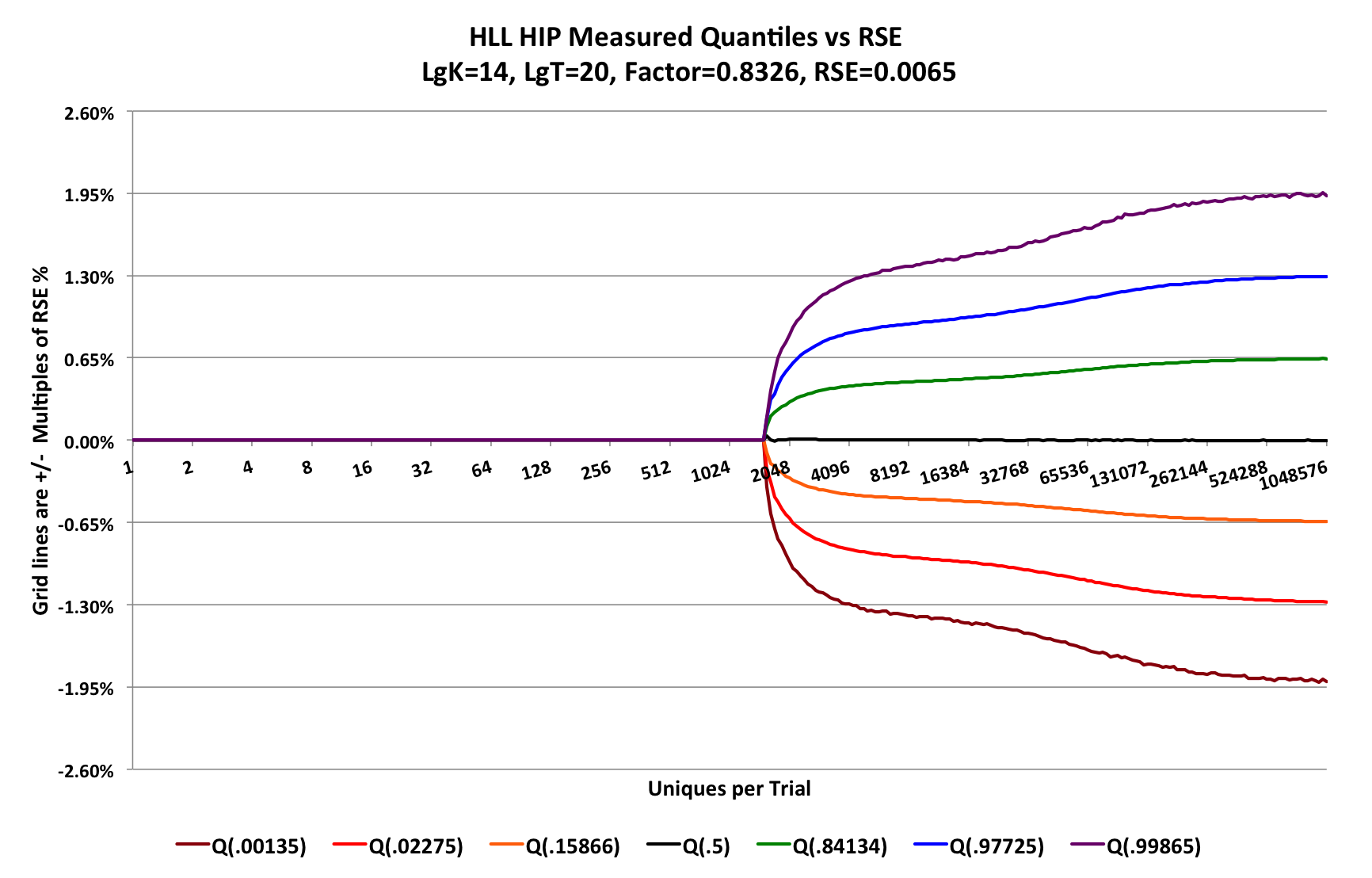
The pitch-fork accuracy plot for any of the HLL sketch types (HLL_4, HLL_6, or HLL_8) are identical because the different sketch types are isomorphic to each other. The following plot was generated with LgK = 14 using 220 trials.

The Factor = 0.8326 is directly relatable to the Flajolet alpha factor of 1.04. As a result, this plot demonstrates that this implementation of the HLL sketch will be about 20% = (0.8326/1.04 - 1) more accurate than a conventional HLL sketch using Flajolet’s estimators (or derived estimators). This is partially due to the use of the HIP estimator1 for range above the transition point, which occurs at about 1500 on the graph. Below this transition point the accuracy is near zero (an RSE of about 50 ppm), which is far better than any known implementation of HLL. This is due to a newly developed theory and estimator developed by Kevin Lang2.
The base Relative Standard Error (RSE) for this sketch (at LgK = 14) is 0.0065 = 0.8326 / sqrt(214). The horizontal gridlines are configured to be +/- multiples of the base RSE.
The different color curves are contours of the actual error distribution measured at normalized rank values derived from the Gaussian distribution at +/- 1, 2, and 3 standard deviations. (See “The Error Distribution Is Not Gaussian” below.)
Therefore, the area between the orange and the green curves represent +/- 1 SD, which corresponds to a confidence level of 68.3%. The area between the red and the blue curves represent +/- 2 SD, which corresponds to a confidence level of 95.4%. The area between the brown and the purple curves represent +/- 3 SD, which correspons to a confidence level of 99.7%.
The reader of this chart can easily see that this size HLL sketch will have error “bounds” of +/- 1.3% with 95.4% confidence. The actual value bounds can also be derived directly from the sketch itself by calling the getUpperBound(numStdDev) and getLowerBound(numStdDev) methods.
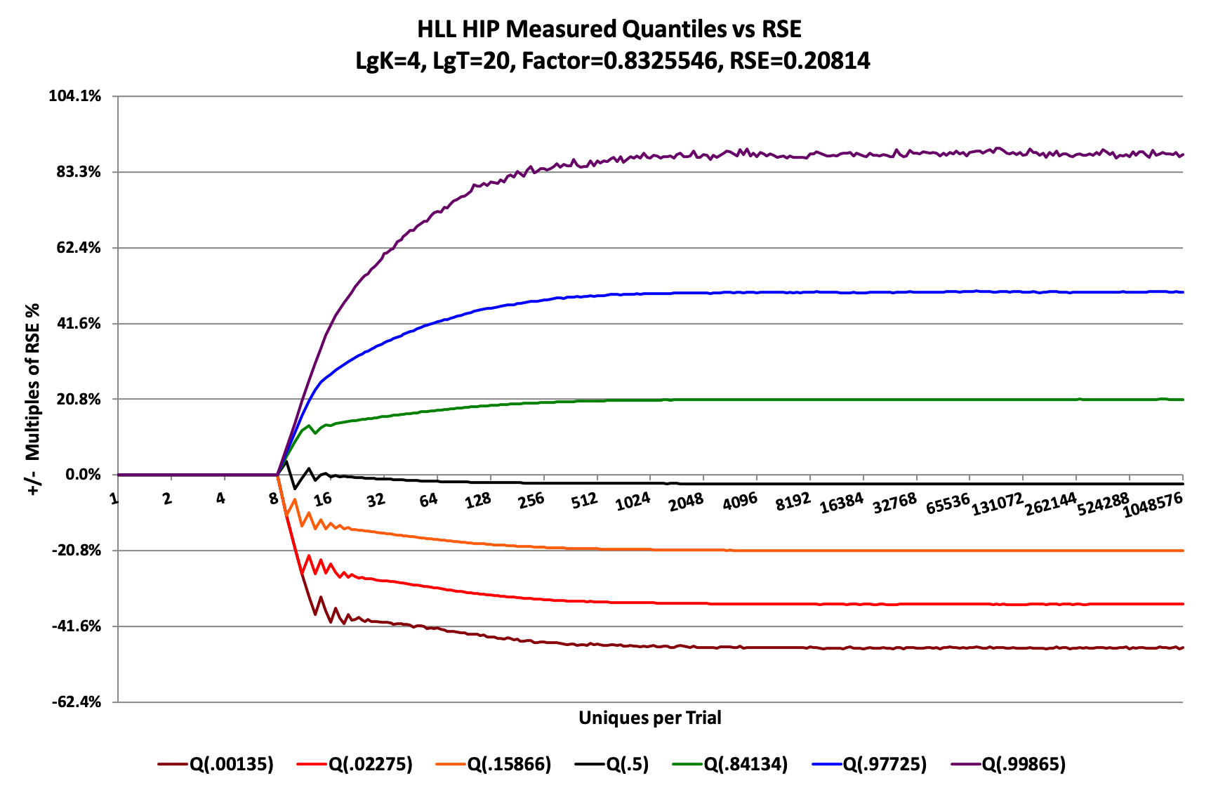
The underlying stochastic processes for unique count sketches (both HLL and Theta) do not produce a symmetric Gaussian error distribution at all. In fact, it is quite complex and more related to the family of multinomial distributions. Nonetheless, the Central Limit Theorem still applies if both K and N are large enough. If K is small (K <= 4096, lgK<=12), and even if N is large, the distribution becomes quite distorted. The following plot for a very small-sized HLL sketch is a good example:

This graph shows the quantile contours for the HLL sketch where LgK = 4 (K = 16). The normalized rank values (the values inside the parentheses, e.g. Q(.00135)) correspond to the normalized rank values at +/- 1,2 and 3 standard deviations of a Gaussian, which this is obviously not! Nonetheless, choosing these quantile points allows us to also claim that the area between the +/- 1 Standard Deviation contours corresponds to 68% confidence; between the +/- 2 Standard Deviation contours corresponds to 95.4% confidence, and between the +/- 3 Standard Deviation contours corresponds to 99.7% confidence. These normalized rank values were chosen because they allow easy comparison with confidence intervals that are commonly used in statistics.
Returning meaningful bounds for low values of K is empirical and approximate. There are no known closed-form mathematical solutions for these error distributions so we use lookup tables and empirical measurements to produce hopefully meaningful bounds.
It is important to understand that the bounds values returned by calling the getUpperBound(numStdDev) and getLowerBound(numStdDev) methods are not hard limits, but attempts to measure meaningful “waist-lines” of distributions that theoretically can reach out to +/- infinity.
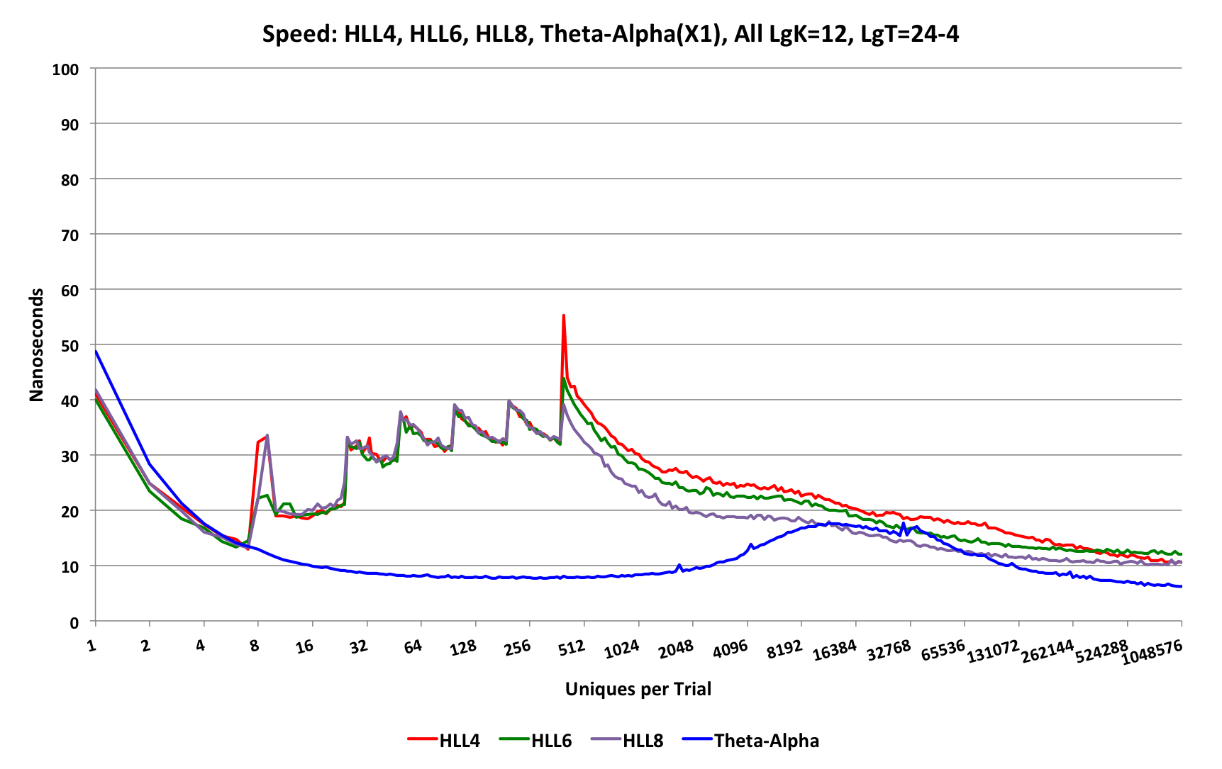
The update speed behavior of the HLL sketches compared to the Theta-Alpha sketch will be similar to the following graph:

The Theta-Alpha sketch is clearly the fastest achieving about 6.5 nanoseconds per update at the high end and staying below 20 nS for nearly the entire range.
All of the HLL types share the same growth strategy below the transition point to the HLL array, which on this graph occurs at about 384 uniques. Above the transition point, the HLL_8 sketch is the fastest followed by the HLL_6 an HLL_4, which are fairly close together.
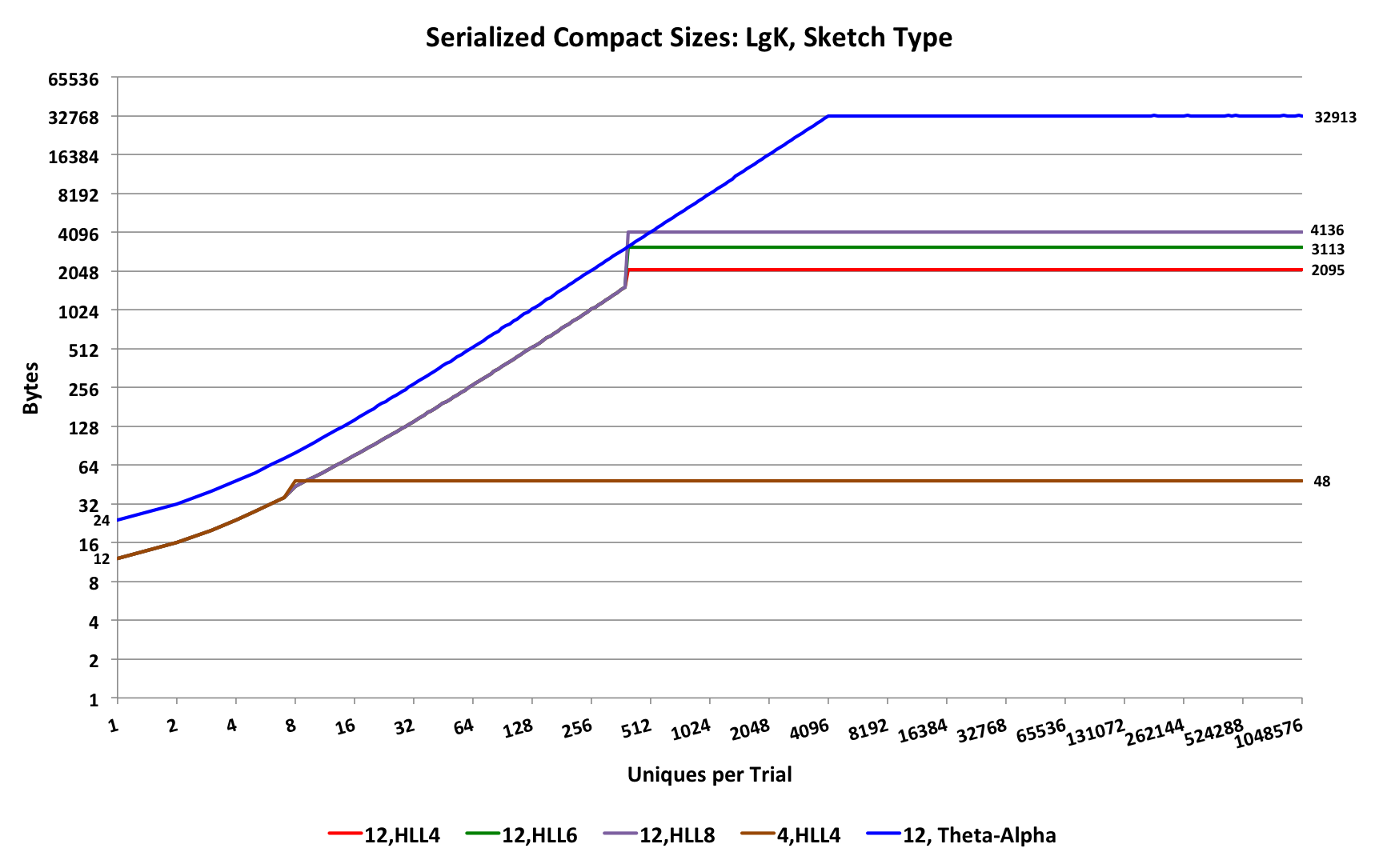
The serialization sizes of the HLL sketches compared to the Theta-Alpha sketch will be similar to the following graph:

Both the HLL sketches and the Theta sketches have a similar growth strategy below their respective transition points.
The HLL sketches grow in increments of 4 bytes, and the Theta sketches grow in increments of 8 bytes.
Thus, below the HLL transition point the Theta sketch is 2X larger than the HLL sketch.
Above the transition point the HLL_4 sketch has a 16X size advantage over the Theta sketch.
Large data with many dimensions and dimension coordinates are often highly skewed creating a “long-tailed” or power-law distribution of unique values per sketch. This can create millions of sketches where a vast majority of the sketches will have only a few entries. It is this long tail of the distribution of sketch sizes that can dominate the overall storage cost for all of the sketches. In this scenario, the size advantage of the HLL can be significantly reduced down to a factor of 2 to 4 compared to Theta sketches. This behavior is strictly a function of the distribution of the input data so it is advisable to understand and measure this phenomenon with your own data.
The HLL sketch is not recommended if you anticipate the need of performing set intersection or difference operations with reasonable accuracy. Instead, use the Theta sketch family.
HLL sketches cannot be intermixed or merged in any way with Theta Sketches.