The up-front / p-sampling option of the Theta Sketches exists to address the system-level storage allocation challenge when dealing with highly partitioned/fragmented massive data that inherently has a long-tail distribution across all the fragments.
Partitioning of Big Data into a large number of fragments will often reveal that the incoming data has a long tail (or, more precisely, a power-law distribution).
For example, Yahoo has a few thousand “properties” and millions of Page-IDs/space-IDs, and users come from many thousands of Where-on-Earth geolocations across the globe. If you were to create a sketch for every dimension-combination of (Page-ID, WOE) you would end up with billions of fragments, each with its own sketch.
As you might expect, you will have a few of those combinations, e.g. (Front-page, New York City) that have very large counts of unique users, and millions of combinations (some small web-app, some small town) that would have only one or 2 users. The sketch automatically limits the number of hashes it keeps for the big combinations to k, while all the hashes are retained for the millions of tiny combinations. When you examine the storage of all those sketches you will discover that roughly 80% of all the storage is consumed by the “degenerate sketches”, which are not sketching at all because they have not received more than k users.
Setting the sampling to, say, p = 0.5, for all sketches, will automatically throw out 50% of all the data coming in to all the sketches. A query against (FP, NYC) will have the same accuracy, with or without the p-sampling, because there is more than enough raw data to fill that sketch. For all the tiny sketches, about half of the ones with only one user hash will disappear. All of the degenerate sketches will be half of their original size when stored. The effect of this is to reduce the overall system-level storage for all sketches by roughly 50%. However, a query against (some small web-app, some small town) may return 0 because it has been “sampled” out. It’s relative error is now infinity! Sketches with more than 1 sample and less the k samples will have error rates that are in-between, but still can be larger than the native RSE of the basic sketch. This effect is illustrated in the following plot, which was created with p=0.5.
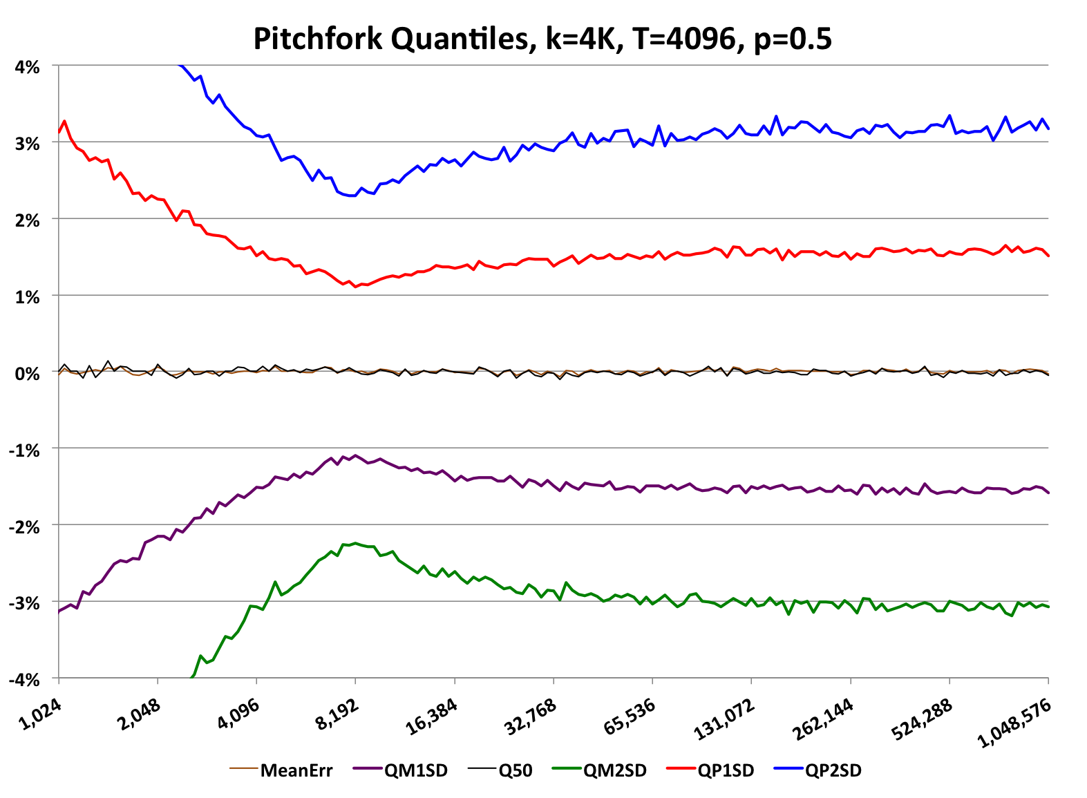
At about 8K uniques there is an inflection point where the error changes direction and begins to increase rather than go toward zero as with the normal pitchfork plots. To the right of this inflection point the error behavior is the same as a normal sketch, with p=1.0, which is the default. To the left of this inflection point the error begins to increase.
The inflection point is the result of two different error behaviors intersecting. To the left of the inflection point the error behavior is that of standard Bernoulli sampling with a fixed probability equal to p. To the right of the inflection point the error behavior is that of the underlying sketch.
The following log-log plot illustrates these intersecting error behaviors more clearly.

The RSE (normalized square-root of the variance) of a Bernoulli sampling process, with fixed p, is a straight line on a log-log plot (plotted in blue). The y intercept at x=1 is simply (1/p -1) and the log-log slope is -1/2. For p=0.5, the y intercept is 1.0 or 100% relative error. So a sketch with only one retained hash value could return estimates of 0, 1 or 2. Although the relative error is large, the absolute error is only +/- 1, which may not be significant.
The green curve represents the theoretical RSE of the sketching process. The red “X” markers are the measured RSE of the combined Bernoulli sampling process and the sketch process.
For p-sampling sketches with very small number of samples the error distribution is very complex and no longer can be modeled with the Gaussian distribution. In order to provide the library user with meaningful getUpperBound() and getLowerBound() values at these very low sample sizes, the library implements more sophisticated error models as illustrated in the following graph.
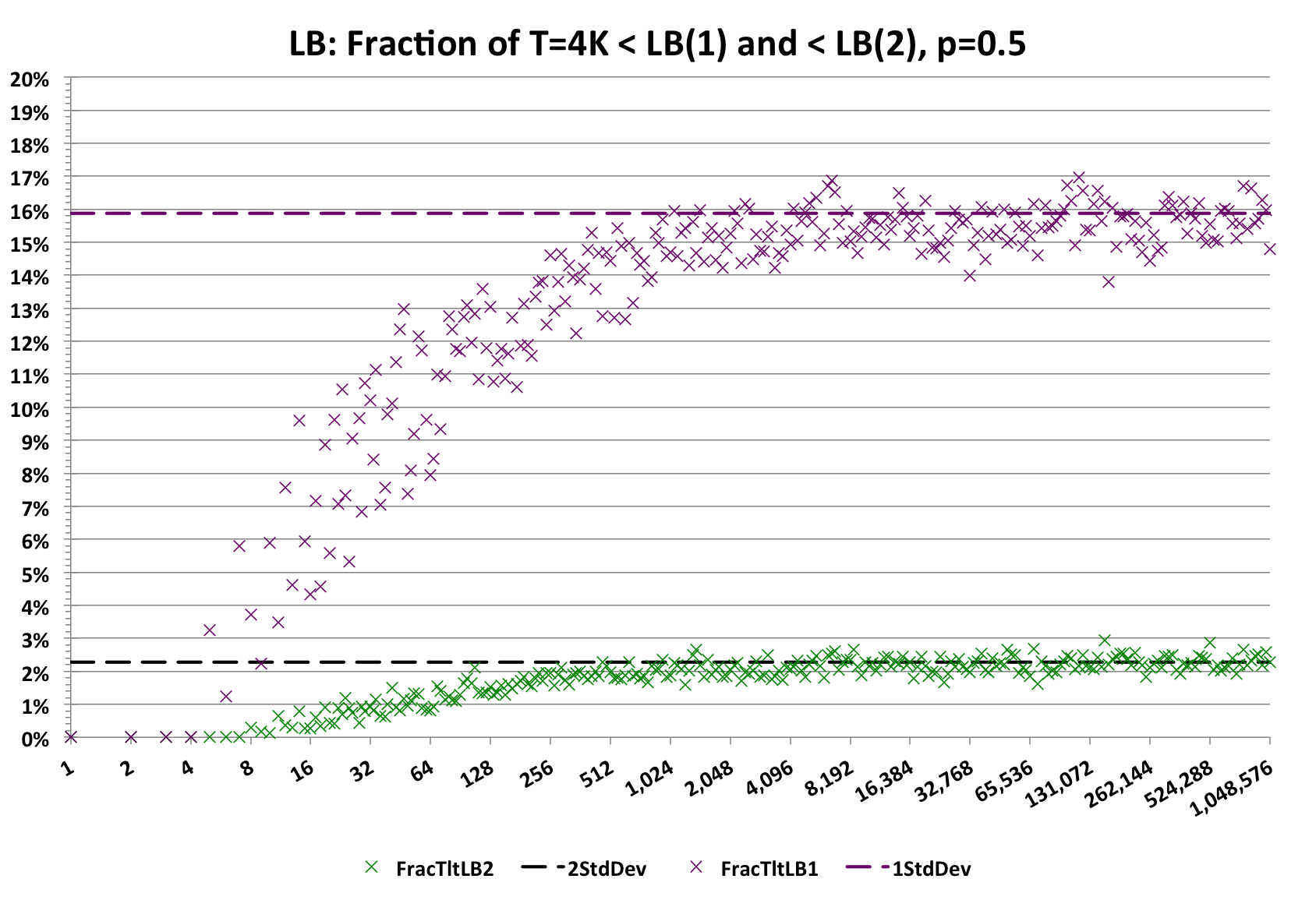
Each point along the X-axis is the result of 4096 trials. The fraction of those 4096 trials that are less than getLowerBound(1) (Purple) should be less than ~16%. The scatter or variance is due to the quantization effects of only 4096 trials. The important thing to note is that for the very low count values, the purple markers are all below the purple dashed line. Similarly, for getLowerBound(2) (Green), the markers should be less than ~2.3%. The graph for the getUpperBound() values is very similar.
As a result of this modeling, the upper and lower bounds values for these very small sample sizes are intentionally conservative. If these bounds had been modeled assuming a Gaussian, the returned values would be way off.
The option of p-sampling provides the systems engineer and product manager with another “knob-to-turn” in trading off overall system storage and acceptable accuracy for small queries. It is quite likely that for the majority of queries, which tend to be against the larger dimension-combinations, the error is quite acceptable. And the product manager may decide that below some threshold size, the small queries have little business value, thus larger error on those queries may be acceptable.
Using this capability must be a carefully thought-through business decision, which is also the case for any form of data sampling.

